In today's world, we are generating lots n lots of data. By 2025, it projected that we will have generated 175 zettabytes of data. But, even though we have so much of data, why is it so difficult to get right data for right model?. Because vast majority of the data being generated is not labeled, and most of the models need labeled data, i.e they use supervised learning. Labeling is an expensive and time consuming job. Many new techniques and Architectures are being developed to overcome this problem like:
All this are extremely interesting and active fields of research. No wonder Yann LeCun, referred to as one of the “Godfather of AI, alongside Geoffrey Hinton & Yoshua Bengio, once said, “most of human and animal learning is unsupervised learning. If intelligence was a cake, unsupervised learning would be the cake, supervised learning would be the icing on the cake, and reinforcement learning would be the cherry on the cake. We know how to make the icing and the cherry, but we don’t know how to make the cake."
Transfer Learning
Transfer Learning is one such technique which helps us in training models using less data and time. Transfer Learning isn’t exactly a ML technique, It is more of a Design Methodology. Creating deep learning models is a tedious process. Trying to train the model from scratch can be very time consuming, the general idea of transfer learning is to reuse the more general patterns learned on some task A and fine-tune it to make it more usable for some task B. This reduces the amount of data needed which is very desirable as getting data requires a lot of expert knowledge. In some cases, transfer learning can also help in getting better results, faster without getting overfitted.
Mathematical Intuition
We know that weight initialization is a very important parameter that we have to take care of while training a model. We have to decide very carefully how we want to initalize them as it can affects the convergence time of the model. Good weight initializations can make the model converge faster and better, and bad ones will take a lot more time to converge or sometimes will not converge at all as they might get stuck in a local minima. Transfer Learning helps us to mitigate the risk of bad convergence. If two tasks Task A and Task B are similar in nature, then, the weights needed for the models will also be similar upto a certain extent. So, instead of randomly intializing the weights, if we resuse the pretrained weights of task A for task B, then, our starting location will be lot better on the cost function terrain, than when we randomly intialize them. This results in faster and better convergence.
It also solves the problem of overfitting as while learning from scratch some patterns might have more influence leading the model to focus on them more and neglecting some other ones, but, in transfer learning due to some pretrained patterns there is good chance that even if the model starts focusing on certain patterns more, the influence of other features or patterns wont decrease by a lot.
Code
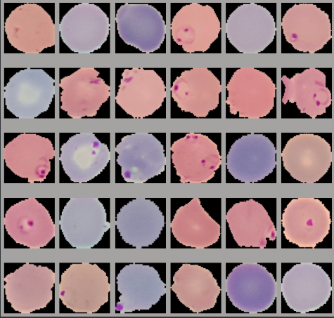
We will be using the malaria dataset provided by tensorflow dataset. For more info: https://www.tensorflow.org/datasets/catalog/malaria.
Importing Libraries
First, we will import the necessary libraries -
import tensorflow as tf
from tensorflow import keras
import numpy as np
import tensorflow_datasets as tfds
import matplotlib.pyplot as plt
import cv2
import os
Defining global variables -
AUTO = tf.data.experimental.AUTOTUNE
DIMS = 128
BATCH_SIZE = 30

os.makedirs("checkpoints/transfer_learning", exist_ok=True)
Pre-Processing the data
The images provided in the dataset do not have the same dimensions, so we will need to convert the images to same dimensions. I decided to convert them to 128x128 size, you may change them if you want. Just remember to accordingly change the input dimensions of the models below.
def get_processed_ds(ds, dims=128, batch_size=None):

    def internal_processing(image_cum_label):
        image = image_cum_label["image"]
        label = image_cum_label["label"]

        image = tf.expand_dims(image, 0)
        image = tf.compat.v1.image.resize_bilinear(image,
                                                   [dims, dims],
                                                   half_pixel_centers=True)
        image = tf.squeeze(image)
        image = tf.cast(image, tf.uint8)
        image = image/255
        return image, label

    ds = ds.map(lambda image_cum_label: internal_processing(image_cum_label),
                num_parallel_calls=AUTO)
    ds = ds.shuffle(20000)
    if batch_size:
        ds = ds.batch(batch_size)
    return ds.prefetch(AUTO)
Now, let’s create train, valid and test datasets -
malaria_train_ds = get_processed_ds(tfds.load("malaria", split="train[:30%]+train[50%:80%]", shuffle_files=True),
                                              dims=DIMS,
                                              batch_size=BATCH_SIZE)
malaria_valid_ds = get_processed_ds(tfds.load("malaria", split="train[30%:40%]+train[80%:90%]", shuffle_files=True),
                                              dims=DIMS,
                                              batch_size=BATCH_SIZE)
malaria_test_ds = get_processed_ds(tfds.load("malaria", split="train[40%:50%]+train[90%:]", shuffle_files=True),
                                             dims=DIMS,
                                             batch_size=BATCH_SIZE)
Let’s look at some of the images -
for item in malaria_train_ds.take(1):
    image_batch, label_batch = item
    print(label_batch)
    fig = plt.figure(figsize=(10, 10))
    rows = 5
    cols = 6
    for i, image in enumerate(image_batch):
        fig.add_subplot(rows, cols, i+1)
        plt.imshow(image)
        plt.axis("off")
plt.tight_layout()
Training the models
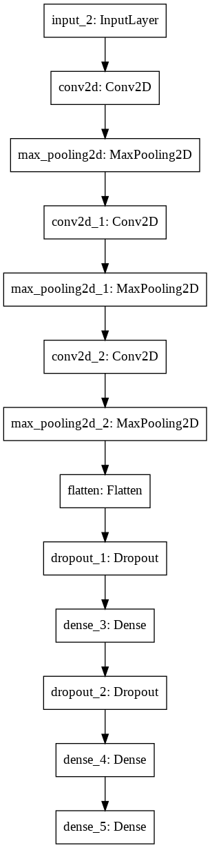
CNN from scratch
We have preprocessed the data, now its time to perform transfer learning experiment. I have used ResNet50 as my pretrained model, you can use any model you like provided its trained on a god amount of data. The ResNet50 backbone used here is trained on the famour ImageNet dataset. Hence, its weights will be a good starting point for our model.
First, We will train a CNN from scratch. Due to the flexibility provided by Tensorflow’s Functional API, I like to write my models using it -
non_tl_input_layer = keras.layers.Input(shape=(DIMS, DIMS, 3))
conv1_layer = keras.layers.Conv2D(64, 3, padding="same", activation="relu")(non_tl_input_layer)
max_pool_1 = keras.layers.MaxPool2D(2)(conv1_layer)
conv2_layer = keras.layers.Conv2D(128, 3, padding="same", activation="relu")(max_pool_1)
max_pool_2 = keras.layers.MaxPool2D(2)(conv2_layer)
conv3_layer = keras.layers.Conv2D(256, 3, padding="same", activation="relu")(max_pool_2)
max_pool_3 = keras.layers.MaxPool2D(2)(conv3_layer)
flatten_layer = keras.layers.Flatten()(max_pool_3)
dp_1 = keras.layers.Dropout(0.1)(flatten_layer)
dense_1 = keras.layers.Dense(512, activation="relu")(dp_1)
dp_2 = keras.layers.Dropout(0.3)(dense_1)
dense_2 = keras.layers.Dense(512, activation="relu")(dp_2)

non_tl_output_layer = keras.layers.Dense(1, activation="sigmoid")(dense_2)

non_tl_model = keras.Model(inputs=[non_tl_input_layer], outputs=[non_tl_output_layer])
non_tl_model.compile(loss=keras.losses.BinaryCrossentropy(),
                     optimizer=keras.optimizers.Nadam(),
                     metrics=["accuracy", "AUC"])
#non_tl_model.summary()
Training the CNN -
non_tl_history = non_tl_model.fit(malaria_train_ds,
                                  validation_data=malaria_valid_ds,
                                  epochs=15,
                                  callbacks=[keras.callbacks.EarlyStopping(patience=5),
                                             keras.callbacks.ModelCheckpoint("checkpoints/transfer_learning/non_tl_model.h5",
                                                                             monitor="val_loss", save_best_only=True, save_weights_only=True,
                                                                             mode='min', save_freq='epoch'),
                                             keras.callbacks.TensorBoard("tensorboards/transfer_learning/non_tl_model")])
np.save("checkpoints/transfer_learning/non_tl_history", non_tl_history.history)
CNN from Scratch:

Epoch 1/15
552/552 [==============================] - 90s 131ms/step - loss: 0.6784 - accuracy: 0.5870 - auc: 0.6207 - val_loss: 0.6413 - val_accuracy: 0.6308 - val_auc: 0.7106
Epoch 2/15
552/552 [==============================] - 84s 128ms/step - loss: 0.6196 - accuracy: 0.6664 - auc: 0.7195 - val_loss: 0.6018 - val_accuracy: 0.6778 - val_auc: 0.7399
Epoch 3/15
552/552 [==============================] - 85s 127ms/step - loss: 0.5764 - accuracy: 0.7093 - auc: 0.7723 - val_loss: 0.4371 - val_accuracy: 0.8041 - val_auc: 0.8932
Epoch 4/15
552/552 [==============================] - 85s 127ms/step - loss: 0.1974 - accuracy: 0.9317 - auc: 0.9760 - val_loss: 0.1478 - val_accuracy: 0.9530 - val_auc: 0.9865
Epoch 5/15
552/552 [==============================] - 85s 127ms/step - loss: 0.1134 - accuracy: 0.9633 - auc: 0.9907 - val_loss: 0.1421 - val_accuracy: 0.9526 - val_auc: 0.9869
Epoch 6/15
552/552 [==============================] - 85s 128ms/step - loss: 0.0752 - accuracy: 0.9753 - auc: 0.9956 - val_loss: 0.1581 - val_accuracy: 0.9530 - val_auc: 0.9841
Epoch 7/15
552/552 [==============================] - 85s 128ms/step - loss: 0.0489 - accuracy: 0.9837 - auc: 0.9978 - val_loss: 0.1807 - val_accuracy: 0.9519 - val_auc: 0.9820
Epoch 8/15
552/552 [==============================] - 84s 127ms/step - loss: 0.0271 - accuracy: 0.9900 - auc: 0.9993 - val_loss: 0.2936 - val_accuracy: 0.9505 - val_auc: 0.9746
Epoch 9/15
552/552 [==============================] - 84s 127ms/step - loss: 0.0249 - accuracy: 0.9921 - auc: 0.9992 - val_loss: 0.2590 - val_accuracy: 0.9456 - val_auc: 0.9759
Epoch 10/15
552/552 [==============================] - 85s 128ms/step - loss: 0.0238 - accuracy: 0.9924 - auc: 0.9991 - val_loss: 0.3091 - val_accuracy: 0.9483 - val_auc: 0.9733

non_tl_model_evaluate: 184/184 [==============================] - 10s 25ms/step - loss: 0.3243 - accuracy: 0.9487 - auc: 0.9730
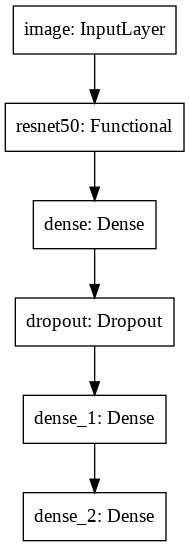
ResNet50 CNN
Now, let’s create a CNN with ResNet50 backbone, we will use the feature vectors from ResNet50 as an input to another layer -
tl_input_layer = keras.layers.Input(shape=(DIMS, DIMS, 3), name="image")
resnet_base = keras.applications.ResNet50(include_top=False,
                                          weights="imagenet",
                                          pooling="avg")(tl_input_layer)
tl_dense_3 = keras.layers.Dense(256, activation="relu")(resnet_base)
dp_3 = keras.layers.Dropout(0.4)(tl_dense_3)
tl_dense_4 = keras.layers.Dense(128, activation="relu")(dp_3)
tl_output_layer = keras.layers.Dense(1, activation="sigmoid")(tl_dense_4)

tl_model = keras.Model(inputs=[tl_input_layer], outputs=[tl_output_layer])
tl_model.compile(loss=keras.losses.BinaryCrossentropy(),
                 optimizer=keras.optimizers.Nadam(),
                 metrics=["accuracy", "AUC"])
#tl_model.summary()
Transfer Learning Using ResNet50:

Epoch 1/15
552/552 [==============================] - 302s 429ms/step - loss: 0.1735 - accuracy: 0.9471 - auc: 0.9804 - val_loss: 0.7167 - val_accuracy: 0.4951 - val_auc: 0.5000
Epoch 2/15
552/552 [==============================] - 247s 423ms/step - loss: 0.1403 - accuracy: 0.9542 - auc: 0.9861 - val_loss: 0.2010 - val_accuracy: 0.9512 - val_auc: 0.9871
Epoch 3/15
552/552 [==============================] - 267s 460ms/step - loss: 0.1270 - accuracy: 0.9574 - auc: 0.9885 - val_loss: 0.1485 - val_accuracy: 0.9574 - val_auc: 0.9871
Epoch 4/15
552/552 [==============================] - 247s 422ms/step - loss: 0.1177 - accuracy: 0.9622 - auc: 0.9899 - val_loss: 0.1839 - val_accuracy: 0.9595 - val_auc: 0.9914
Epoch 5/15
552/552 [==============================] - 247s 423ms/step - loss: 0.1125 - accuracy: 0.9618 - auc: 0.9910 - val_loss: 0.1363 - val_accuracy: 0.9597 - val_auc: 0.9904
Epoch 6/15
552/552 [==============================] - 247s 423ms/step - loss: 0.1060 - accuracy: 0.9630 - auc: 0.9919 - val_loss: 0.2520 - val_accuracy: 0.9546 - val_auc: 0.9849
Epoch 7/15
552/552 [==============================] - 248s 423ms/step - loss: 0.1042 - accuracy: 0.9629 - auc: 0.9923 - val_loss: 0.2675 - val_accuracy: 0.9510 - val_auc: 0.9768
Epoch 8/15
552/552 [==============================] - 246s 422ms/step - loss: 0.1002 - accuracy: 0.9641 - auc: 0.9929 - val_loss: 1.5985 - val_accuracy: 0.7453 - val_auc: 0.8417
Epoch 9/15
552/552 [==============================] - 248s 423ms/step - loss: 0.1030 - accuracy: 0.9629 - auc: 0.9926 - val_loss: 0.1869 - val_accuracy: 0.9603 - val_auc: 0.9902
Epoch 10/15
552/552 [==============================] - 248s 424ms/step - loss: 0.0924 - accuracy: 0.9680 - auc: 0.9940 - val_loss: 0.1613 - val_accuracy: 0.9579 - val_auc: 0.9862

TL_model_evaluate: 184/184 [==============================] - 24s 94ms/step - loss: 0.1630 - accuracy: 0.9554 - auc: 0.9863
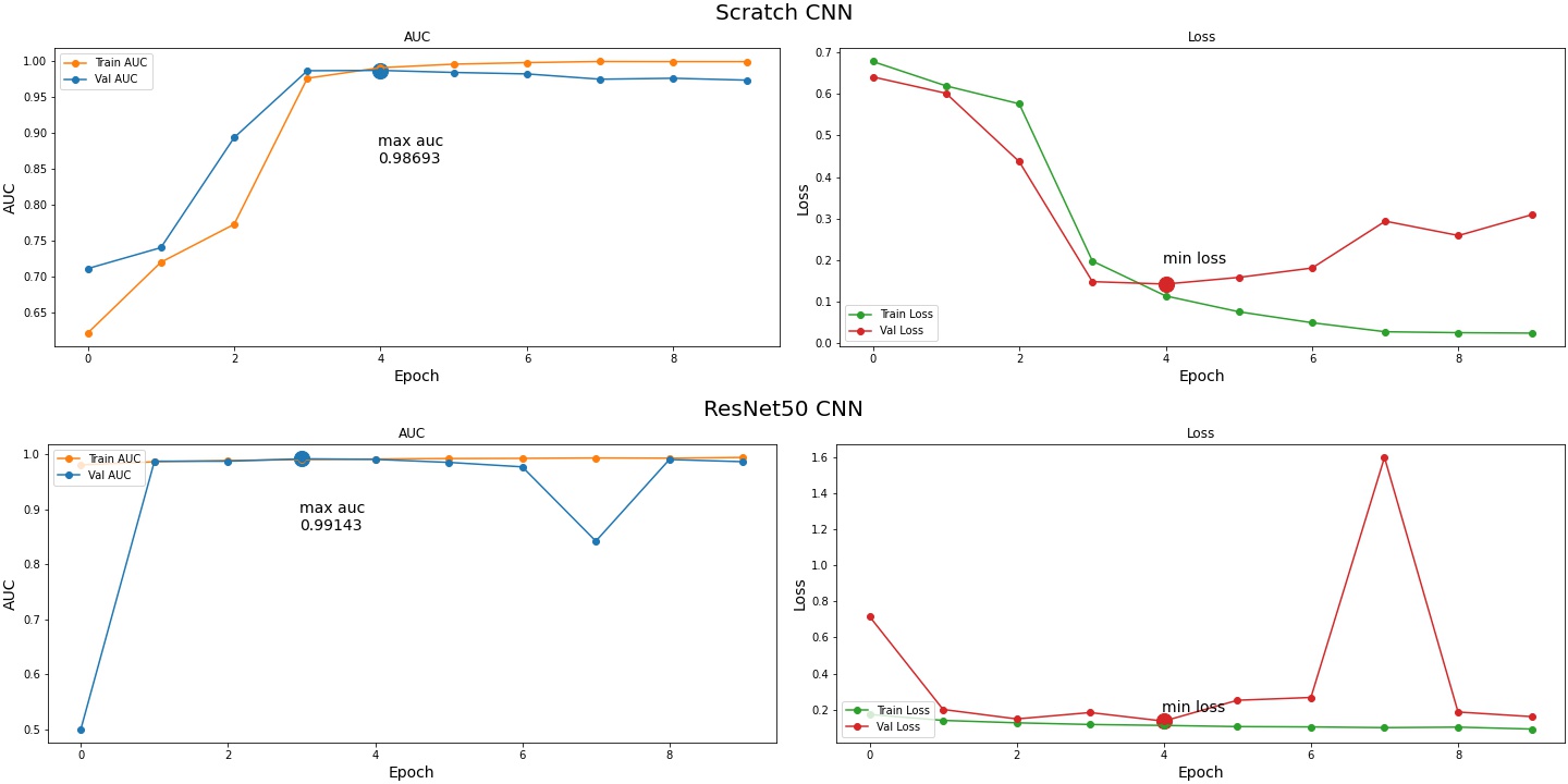
Results
THANKS FOR READING!!